Restricted cubic splines
Shengping Yang PhD
Corresponding author: Shengping Yang
Contact Information: Shengping.Yang@PBRC.org
DOI: 10.12746/swjm.v14i60.1679
I am using linear regression to evaluate the association between body fat percentage and HbA1c; however, I am uncertain whether this relationship is truly linear. I am therefore considering whether restricted cubic splines (RCS) may provide a more appropriate approach for modeling this association.
Regression models are widely used to estimate relationships between predictors and outcomes. A key challenge arises when modeling continuous predictors, for which the true functional form is often unknown. Analysts must balance model simplicity with the need to accurately capture potentially complex relationships. Traditional approaches include categorizing continuous variables or applying polynomial transformations, although other methods such as fractional polynomials, generalized additive models, and piecewise regression are also available.
1. LIMITATIONS OF TRADITIONAL MODELING APPROACHES
1.1 CATEGORIZING CONTINUOUS VARIABLES
A common but suboptimal approach to handling continuous predictors is categorization (e.g., grouping age or body mass index into intervals). Although convenient, this practice introduces several well-documented limitations:
- Loss of information and statistical power
Categorization discards within-group variability, reducing statistical efficiency and the ability to detect true associations.
- Artificial discontinuities
Categorized models assume constant risk within intervals and abrupt changes at cut points, resulting in unrealistic step functions that poorly reflect biological processes.
- Arbitrary threshold selection
Cut points are often chosen without strong theoretical justification. Different choices can yield different conclusions, increasing the risk of biased or non-reproducible results.
- Masking of non-linear relationships
Important patterns, such as U-shaped or threshold effects, may be obscured when continuous variables are coarsely grouped.
1.2 POLYNOMIAL MODELS
Polynomial regression offers a more flexible alternative by allowing curved relationships; however, it also has notable drawbacks:
- Global influence of higher-order terms
Polynomial functions are sensitive to extreme values, and higher-order terms can produce unstable estimates, particularly near the boundaries of the data.
- Poor interpretability
Coefficients of higher-order terms are difficult to interpret meaningfully.
- Risk of overfitting
High-degree polynomials may fit observed data well but perform poorly in new samples.
- Unrealistic functional forms
Polynomials can impose oscillatory or exaggerated curvature that does not reflect the true underlying relationship.
To address these limitations, restricted cubic splines (RCS) are often used.
2. RESTRICTED CUBIC SPLINES
Restricted cubic splines provide a flexible approach for modeling non-linear effects without imposing strong parametric assumptions. They model continuous predictors using piecewise cubic polynomials joined at predefined values (knots). These polynomials are constrained to ensure a smooth and continuous fitted curve, including continuity of the first and second derivatives.1,2
Importantly, RCS imposes linearity beyond the boundary knots, which stabilizes the model in regions with sparse data. Rather than fitting separate independent curves, spline basis functions collectively define a single smooth function across the predictor’s range. This approach preserves information while allowing flexible, data-driven estimation of non-linear relationships.3
2.1 KEY FEATURES OF RCS
2.1.1 CORE COMPONENTS
An RCS model consists of three elements:
- Linear base: The model includes a linear term for the predictor.
- Cubic flexibility: Cubic polynomials allow curvature between knots.
- Restriction: The function is constrained to be linear before the first knot and after the last knot, preventing instability at the tails.
2.1.2 KNOTS
Knots are the points at which the functional form changes. They are typically at fixed quantiles of the predictor (e.g., 5th, 35th, 65th, and 95th percentiles for four knots), and act as ‘hinges’ or transition points where the mathematical description of the relationship is allowed to change to better fit local data trends.
2.1.3 BASIS FUNCTIONS
The basis functions are the transformed version of X. Instead of modeling a continuous predictor X directly, these functions are constructed to fit the data so that curvature vanishes beyond the last knot, ensuring linear tails. For an RCS with k knots, there are k basis functions - Basis 1 is the linear term X, and the remaining bases are the non-linear transformations that introduce curvature.
2.2 PIECEWISE POLYNOMIAL INTERPRETATION
Although implemented using basis functions, the fitted model can be understood as a series of piecewise polynomials:
2.2.1 NUMBER OF SEGMENTS
There are a total of k + 1 segments - one before the first knot; k − 1 between knots; and one after the last knot.
2.2.2 FORM OF SEGMENTS
The first and the last segments are linear and the segments in between are cubic. In addition, at each knot, adjacent segments share the same value, slope (first derivative), and curvature (second derivative), ensuring smoothness.
2.3 MATHEMATICAL FORMULATION
For a predictor X with knots k1, k2, … , km, the spline function can be written as:

Where βj s are the estimated parameters, Bj(X)s are the spline basis functions and f(X) is the estimated relationship.
3. ILLUSTRATIVE EXAMPLE
To illustrate RCS, consider the relationship between a continuous predictor X and an outcome Y. Figure 1 demonstrates three complementary views of this modeling approach - specifically, how RCS differs from unrestricted piecewise polynomials, and how basis functions look like and constructed to fit the data.
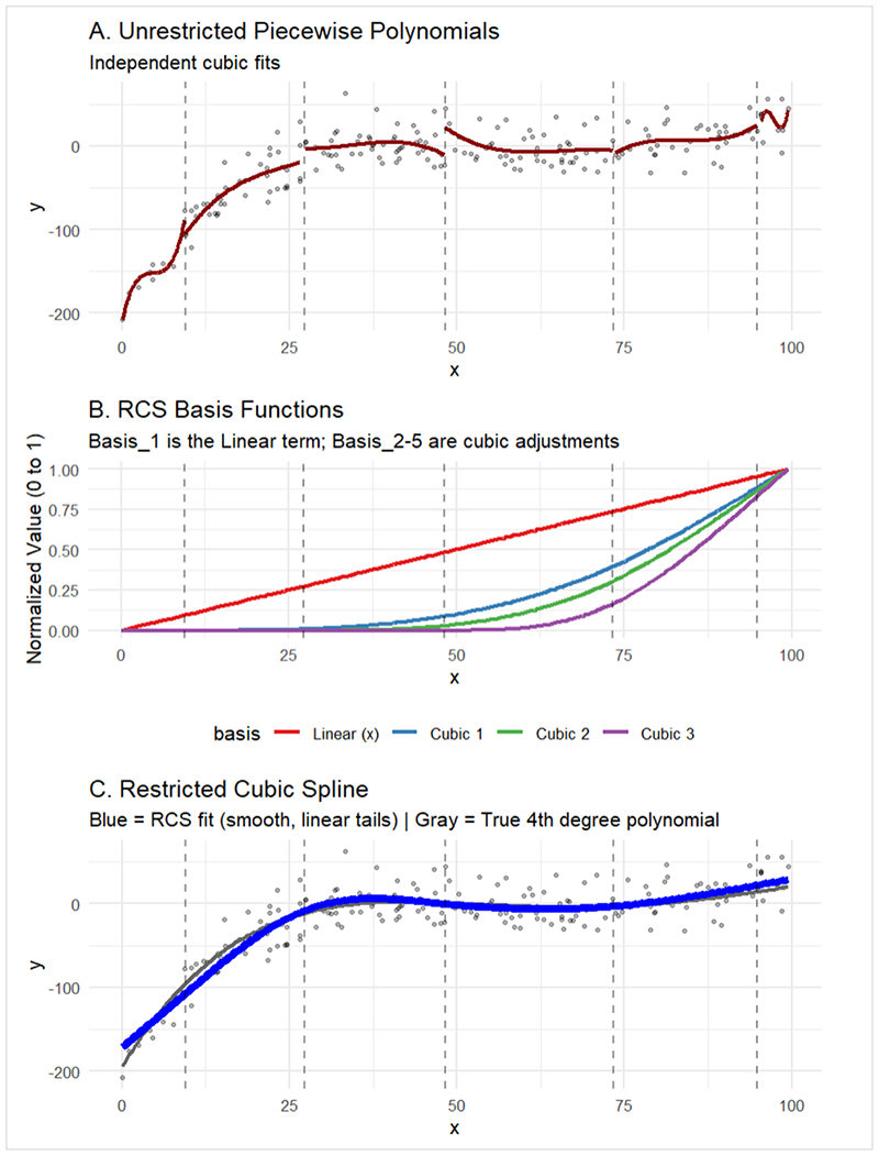
Figure 1. A: Unrestricted polynomial; B: The RCS basis functions; C: The RCS fit in blue, with the 4th degree polynomial fit in gray (the true model).
Because RCS is a special form of piecewise polynomials, we start with evaluating unrestricted form of piecewise polynomial.
3.1 UNRESTRICTED PIECEWISE POLYNOMIALS
The knots are defined as the 5th, 25th, 50th, 75th and 95th quartiles (the vertical dashed lines). Independent cubic polynomials are fitted within each interval defined by knots. While each segment fits local data well, there are obvious discontinuities (“jumps”) occurring at the knots, highlighting a major limitation of this approach (Figure 1A).
3.2 RCS FIT
3.2.1 THE BASIS FUNCTIONS
The same knots are defined for RCS, and the RCS model is decomposed into five basis functions - Basis 1 determines the linear trend and Bases 2-5 are used for making non-linear adjustments
It is worth noting that Bases 2-5 are cubic functions specifically engineered to have zero value and zero slope before they reach their respective knots. Once they pass a knot, they introduce a cubic curvature to “bend” the total model. In addition, those curves often look somewhat quadratic at first glance (Figure 1B; Bases 2-5), which is due to the “Restriction” component, including: (a) RCS is forced to be linear beyond the final boundary knot. To achieve this, the Basis functions are mathematically constructed so that their second and third derivatives cancel out after the last knot; (b) They must maintain continuity of the first and second derivatives at every knot - you don’t see the sharp “turns” or the dramatic “tails” associated with a standard cubic function; and (c) These functions are meant to be added together. A single basis function might look like a simple curve, but when weighted by its coefficient and added to the linear term, it allows the final model to fit complex, non-linear patterns like U-shapes or plateaus. In other words, these functions activate progressively at their respective knots, contributing to the overall shape of the curve (Figure 1B). Another reason these functions look somewhat quadratic is that the figure does not cover the full range of the functions.
3.2.2 THE RCS CURVE
The weighted sum of the Basis functions produces a single smooth curve (Figure 1C). Importantly, this curve remains linear at both tails and has smooth connections between local curves. By using a 5-knot RCS, the fitted curve closely approximates the true underlying relationship, which is an underlying 4th degree polynomial (the gray curve). Compared with unrestricted piecewise polynomials (Figure 1A), RCS eliminates discontinuities and avoids unrealistic oscillations. The linear tails improve stability where data are sparse.4,5
4. IMPLEMENTATION CONSIDERATIONS
There are a few considerations when implementing RCS.6
4.1 CHOOSING THE NUMBER OF KNOTS
The number of knots determines flexibility:
- 3 knots: Simple curvature (e.g., U-shaped)
- 4 knots: Recommended starting point
- 5 knots: More complex relationships
- 6-7 knots: Only for large samples (e.g., n > 500)
A useful rule of thumb is to limit non-linear degrees of freedom (the number of independent parameters used to model a relationship) to approximately n/30 to n/20.
4.2 KNOT PLACEMENT STRATEGIES
There are a few options for choosing the locations of the knots.
- Quantile-based: Knots are typically placed at fixed quantiles of the predictor distribution. Their number and placement determine model flexibility (Too few knots often resulted in underfitting; Too many knots often resulted in overfitting).
- Equally spaced: Based on the predictor range (might be a concern if there are outlying values in X).
- Clinically informed: Based on meaningful thresholds.
4.3 TESTING FOR NON-LINEARITY
To formally evaluate whether an RCS model is better than a linear model, a test on non-linearity can be performed using:
- Wald test (non-linear terms = 0)
- Likelihood ratio test (linear vs spline model)
- Information criteria (AIC/BIC)
5. THE ADVANTAGES OF RCS
Restricted cubic splines address several key limitations of traditional approaches to modeling continuous predictors (Table 1). First, unlike categorization, RCS preserves the full information contained in continuous variables, thereby maintaining statistical power and avoiding arbitrary cut points. At the same time, they provide substantially greater flexibility than simple linear models, allowing the data to determine the shape of the association without imposing unrealistic assumptions. In contrast to high-degree polynomials, which can be overly sensitive to extreme values and prone to erratic behavior at the boundaries, RCS enforce linearity in the tails. This constraint improves model stability and reduces the risk of implausible extrapolation in regions with sparse data.
Table 1. Comparison of Features
| Feature |
Traditional Categorization |
Polynomial Regression |
Restricted Cubic Splines |
| Preserves continuous nature |
NO |
YES |
YES |
| Local flexibility |
NO |
NO |
YES |
| Stable tails |
N/A |
NO |
YES |
| Interpretable coefficients |
NO |
NO |
YES* |
| No arbitrary cutpoints |
NO |
YES |
YES |
In addition, RCS produce smooth, continuous functions that better reflect biological and clinical processes than step functions or oscillatory polynomial curves. Although individual spline coefficients are not directly interpretable, the overall fitted relationship can be readily visualized, facilitating identification of clinically meaningful patterns such as thresholds, plateaus, or non-monotonic associations. Importantly, RCS can be implemented within standard regression frameworks, such as ordinary linear regression, logistic regression and cox regression,7,8 etc., enabling adjustment for confounders and formal testing of non-linearity (e.g., via Wald or likelihood ratio tests). Together, these properties make RCS a flexible, robust, and interpretable approach for modeling complex predictor-outcome relationships while avoiding the key pitfalls outlined in Table 1.
In summary, RCS offer a flexible approach for modeling non-linear associations between continuous predictors and outcomes without the rigid assumptions of simple linear models or the instability of high-order polynomials. By utilizing piecewise cubic polynomials joined at knots, RCS can capture complex, local data trends such as U-shaped relationships or plateaus while ensuring a smooth, continuous fitted curve. The application of RCS on studies such as the relationship between body fat percentage and HbA1c would be an ideal practice. A defining feature of RCS is the restriction of the function to be linear beyond the outer boundary knots, which significantly improves model stability and prevents unrealistic oscillations in regions with sparse data. When implementing RCS, analysts typically use 3 to 5 knots placed at quantile-based locations to balance model flexibility with the risk of overfitting.
REFERENCES
- Durrleman S, Simon R. Flexible regression models with cubic splines. Stat Med. 1989 May;8(5):551-61.
- Belias M, Rovers MM, Hoogland J, Reitsma JB, Debray TPA, IntHout J. Predicting personalised absolute treatment effects in individual participant data meta-analysis: An introduction to splines. Res Synth Methods. 2022 Mar;13(2):255-83.
- Lusa L, Ahlin Č. Restricted cubic splines for modelling periodic data. PLoS ONE. 2020;15(10):e0241364.
- Gauthier J, Wu QV, Gooley TA. Cubic splines to model relationships between continuous variables and outcomes: a guide for clinicians. Bone Marrow Transplant. 2020 Apr;55(4):675-80. doi: 10.1038/s41409-019-0679-x. Epub 2019 Oct 1. Erratum in: Bone Marrow Transplant. 2023 Aug;58(8):962.
- Orsini, N, Greenland, S. A Procedure to Tabulate and Plot Results after Flexible Modeling of a Quantitative Covariate. The Stata Journal: Promoting communications on statistics and Stata. 2011;11(1):1-29.
- Arnes JI, Hapfelmeier A, Horsch A, Braaten T. Greedy knot selection algorithm for restricted cubic spline regression. Front Epidemiol. 2023 Dec 18;3:1283705.
- Austin PC. Graphical methods to illustrate the nature of the relation between a continuous variable and the outcome when using restricted cubic splines with a Cox proportional hazards model. Stat Methods Med Res. 2025 Feb;34(2):277-85. Epub 2024 Oct 21.
- Desquilbet L, Mariotti F. Dose-response analyses using restricted cubic spline functions in public health research. Stat Med. 2010 Apr 30;29(9):1037-57.
Article citation: Yang S. Restricted cubic splines. The Southwest Journal of Medicine. 2026;14(60):90-95
From: Department of Biostatistics, Pennington Biomedical Research Center, Baton Rouge, LA (SY)
Conflicts of interest: none
This work is licensed under a Creative Commons Attribution-ShareAlike 4.0 International License.